amep.spatialcor.sfiso

amep.spatialcor.sfiso(coords: ndarray, box_boundary: ndarray, N: int, qmax: float = 20.0, twod: bool = True, njobs: int = 1, chunksize: int | None = None, mode: str = 'std', other_coords: ndarray | None = None, accuracy: float = 0.5, num: int = 64, verbose: bool = False) → tuple[ndarray, ndarray]

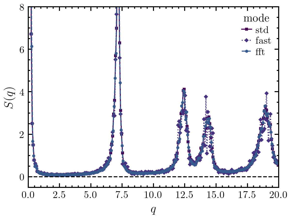
Calculates the isotropic static structure factor for a given set of coordinates.

Notes

The isotropic static structure factor is defined by

\[S_{3D}(q) = \frac{1}{N}\left\langle\sum_{m,l=1}^N\frac{\sin(qr_{ml})}{qr_{ml}}\right\rangle\]

\[S_{2D}(q) = \frac{1}{N}\left\langle\sum_{m,l=1}^N J_0(qr_{ml})\right\rangle\]

with \(r_{ml}=|\vec{r}_m-\vec{r}_l|\) and the Bessel function of the first kind \(J_0(x)\).

For mode=’fast’, a rewritten form for homogeneous and isotropic systems is used that reduces the number of computations from \(\mathcal{O}(N^2)\) to \(\mathcal{O}(N)\), where \(N\) is the number of particles [1].

Mode ‘fft’ only works in 2D!!!

References

[1]

Aichele, M., & Baschnagel, J. (2001). Glassy dynamics of simulated polymer melts: Coherent scattering and van Hove correlation functions. The European Physical Journal E, 5(2), 229–243. https://doi.org/10.1007/s101890170078

Parameters:

• coords (np.ndarray of shape (N,3)) – Coordinates.

• (3 (np.ndarray of shape) – Boundary of the simulation box in the form of np.array([[xmin, xmax], [ymin, ymax], [zmin, zmax]])

• 2) – Boundary of the simulation box in the form of np.array([[xmin, xmax], [ymin, ymax], [zmin, zmax]])

• N (int) – Total number of particles.

• qmax (float, optional) – Maximum wave number to consider. The default is 20.

• twod (bool, optional) – If True, the 2D form is used. The default is True.

• njobs (int, optional) – Number of jobs for multiprocessing. The default is 1.

• chunksize (int, optional) – In ‘std’ mode, the calculation is divided into chunks of this size. The default is 1000.

• mode (str, optional) – One of [‘std’, ‘fast’, ‘fft’]. The ‘fft’ mode only works if twod is True. The default is ‘std’.

• other_coords (np.ndarray, optional) – Coordinate frame of the other species to which the correlation is calculated. The default is None (uses coords).

• accuracy (float, optional) – Accuracy for fft mode. 0.0 means least accuracy, 1.0 best accuracy. The default is 0.5. Note that a higher accuracy needs more memory for the computation. accuracy must be in (0,1].

• num (int, optional) – Number of q vectors to average over in ‘fast’ mode. If twod is False, the number of q vectors is equal to num^2. The default is 64.

• verbose (bool, optional) – If True, additional information is printed and a progress bar is shown. The default is False.

Returns:

• S (np.ndarray) – Isotropic static structure factor.

• q (np.ndarray) – Wave numbers.

Examples

>>> import amep
>>> traj = amep.load.traj("../examples/data/lammps.h5amep")
>>> frame = traj[-1]
>>> S0, q0 = amep.spatialcor.sfiso(
...     frame.coords(), frame.box, frame.n(),
...     njobs=6, twod=True, chunksize=1000, mode='std'
... )
>>> S1, q1 = amep.spatialcor.sfiso(
...     frame.coords(), frame.box, frame.n(),
...     njobs=6, twod=True, chunksize=1000, mode='fast'
... )
>>> S2, q2 = amep.spatialcor.sfiso(
...     frame.coords(), frame.box, frame.n(),
...     njobs=6, twod=True, chunksize=1000, mode='fft', accuracy=0.5
... )
>>> fig, axs = amep.plot.new()
>>> axs.plot(q0, S0, ls='-', label='std')
>>> axs.plot(q1, S1, ls=':', label='fast')
>>> axs.plot(q2, S2, ls='--', label='fft')
>>> axs.set_ylim(-0.5, 8)
>>> axs.set_xlim(0, 20)
>>> axs.legend(title='mode')
>>> axs.set_xlabel(r'$q$')
>>> axs.set_ylabel(r'$S(q)$')
>>> axs.axhline(0, c='k', ls='--', lw=1)
>>> fig.savefig('./figures/spatialcor/spatialcor-sfiso.png')
>>>