amep.continuum.sf2d

amep.continuum.sf2d(dfield: ndarray, X: ndarray, Y: ndarray, other_dfield: ndarray | None = None, Ntot: int | None = None, njobs: int = 1) → tuple[ndarray, ndarray, ndarray]

Calculate the 2D static structure factor from a density field.

Is done via Fourier transform.

Notes

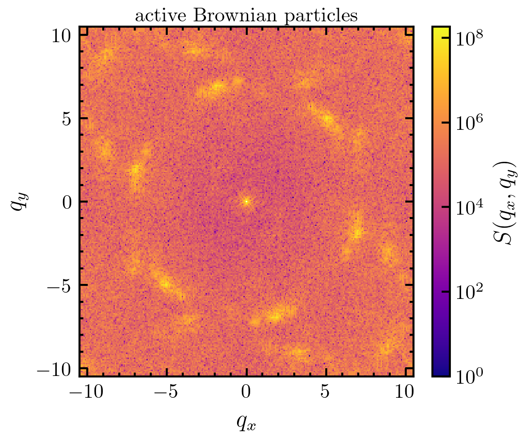
The static structure factor is defined by

\[S(\vec{q}) = <\rho(\vec{q})\rho(\vec{-q})>= <|\rho(\vec{q})|^2>,\]

where $rho(vec{q})$ is the Fourier transform of the particle number density (see Ref. [1] [2] [3] for further information).

[1]

Hansen, J.-P., & McDonald, I. R. (2006). Theory of Simple Liquids (3rd ed.). Elsevier. https://doi.org/10.1016/B978-0-12-370535-8.X5000-9 (p. 78 and 83)

[2]

Bray, A. J. (1994). Theory of phase-ordering kinetics. Advances in Physics, 43(3), 357–459. https://doi.org/10.1080/00018739400101505

[3]

Wittkowski, Raphael, et al. “Scalar φ 4 field theory for active-particle phase separation.” Nature communications 5.1 (2014): 4351. https://doi.org/10.1038/ncomms5351

S(0,0) is set to 0

Parameters:

• dfield (np.ndarray) – Two dimensional density field.

• X (np.ndarray) – x coordinates of grid cells in form of a meshgrid with same shape as dfield.

• Y (np.ndarray) – y coordinates of grid cells in form of a meshgrid with same shape as dfield.

• other_dfield (np.ndarray, optional) – Two dimensional density field to which the correlation should be calculated. The default is None (use dfield).

• Ntot (int, optional) – Total number of particles in the system. This value is needed for the correct normalization of the structure factor. If None, Ntot is calculated from the integral over dfield. The default is None.

• njobs (int, optional) – Number of processors used for the parallel computation of the fft. The default is 1.

Returns:

• np.ndarray – 2d static structure factor.

• np.ndarray – x components of the wave vectors.

• np.ndarray – y components of the wave vectors.

Examples

>>> import amep
>>> import matplotlib as mpl
>>> traj = amep.load.traj("../examples/data/lammps.h5amep")
>>> frame = traj[-1]
>>> d, X, Y = amep.continuum.coords_to_density(
...     frame.coords(), frame.box, dmin=0.3
... )
>>> S, Kx, Ky = amep.continuum.sf2d(d, X, Y)
>>> fig, axs = amep.plot.new(figsize=(3.6,3))
>>> mp = amep.plot.field(
...     axs, S, Kx, Ky, cscale="log", vmin=1e0
... )
>>> cax = amep.plot.add_colorbar(
...     fig, axs, mp, label=r"$S(q_x,q_y)$"
... )
>>> axs.set_xlabel(r'$q_x$')
>>> axs.set_ylabel(r'$q_y$')
>>> axs.set_title(r"active Brownian particles")
>>> fig.savefig('./figures/continuum/continuum-sf2d_1.png')

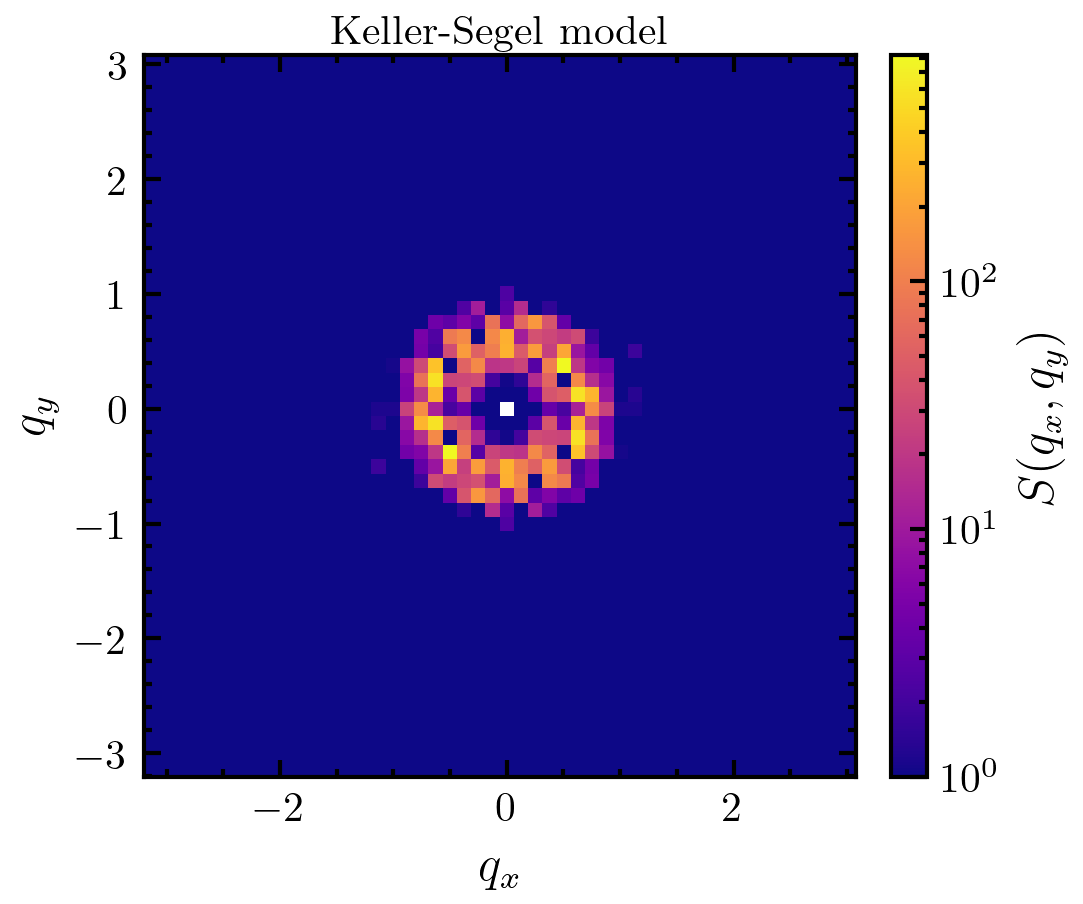
>>> traj = amep.load.traj("../examples/data/continuum.h5amep")
>>> frame = traj[3]
>>> S, Kx, Ky = amep.continuum.sf2d(
...     frame.data("p"), *frame.grid
... )
>>> fig, axs = amep.plot.new(figsize=(3.6,3))
>>> mp = amep.plot.field(
...     axs, S, Kx, Ky, cscale="log", vmin=1e0
... )
>>> cax = amep.plot.add_colorbar(
...     fig, axs, mp, label=r"$S(q_x,q_y)$"
... )
>>> axs.set_xlabel(r'$q_x$')
>>> axs.set_ylabel(r'$q_y$')
>>> axs.set_title(r"Keller-Segel model")
>>> fig.savefig('./figures/continuum/continuum-sf2d_2.png')